Excel Dropdown List
In this tutorial, I will show you how to make dropdown list in Excel with examples. Not only will I show you ways of how to create dropdown but how to use its values in different formulas as well.
The dropdown in Excel is useful if you require restricting users selecting a value from the predefined set of list. For example, you require users selecting a color from the limited options in a cell:
- Black
- Blue
- Red
- Green
To ensure that, you may add a dropdown in the Excel sheet in a specific cell quite easily. In this tutorial, I will show you how to make dropdown list in Excel with examples. Not only will I show you ways of how to create dropdown but how to use its values in different formulas as well.
Steps of Adding a dropdown list in Excel
Inserting a dropdown in sheet’s cell is pretty simple. Just follow these simple steps for creating a Color dropdown:
Step 1:
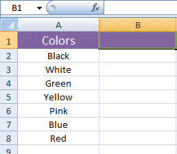
Add the color names in cells. For the demo, I have added seven colors to the column A2 to A8:
Step 2:
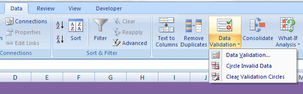
Select the cell where you want to create a dropdown. I selected B1. Now go to the Data in the Ribbon and press the “Data Validation” as shown below.
Step 3:
The “Data Validation” dialog should appear.
We will explore different options, first let met create a dropdown with color values quickly.
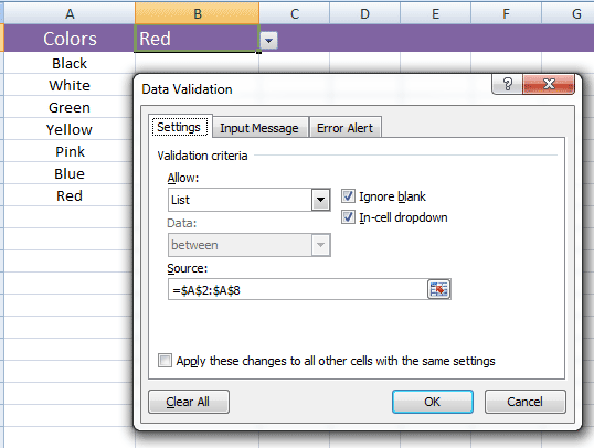
In the “Data Validation” dialog, press the “Allow” dropdown and choose “List” option.
You should see the “Source” text box. Enter the following formula:
=$A$2:$A$8
And keep the “Ignore Blank” and “In cell dropdown” checkboxes checked. Press “OK”.
A dropdown should be created in the selected cell (B1) as shown below:
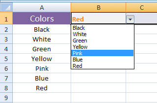
Is not that so simple?
Add a dropdown without cell values example
As our previous dropdown is based on the formula that refers cells A2 to A8. If you change the values there, the dropdown list will also change accordingly. For example, if I change the color from “Yellow” to “Cyan”, the dropdown will also reflect this.
What if you want to create a dropdown with its own list of options – independent of cells?
Again, pretty simple. Follow these steps:
- Select the cell where you want to create the dropdown.
- Open the Data -> Data Validation (like in previous example)
- In the Data Validation dialog, select the List in “Allow” dropdown.
- In the source textbox, just enter the color names (or any options that you need in the dropdown) and separate each option by a comma (as shown below)
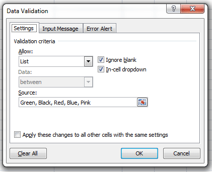
- Press OK.
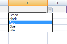
A dropdown should be created as shown below:
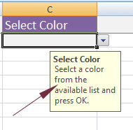
Showing input message for dropdown example
If you want to display a message when the cell is selected containing a dropdown then you may also display a descriptive message as shown below:
Follow these steps for making a dropdown with input message.
I am assuming, you already created a dropdown. Select that dropdown and open the Data --> Data Validation dialog.
Select the “Input Message” tab as shown below:
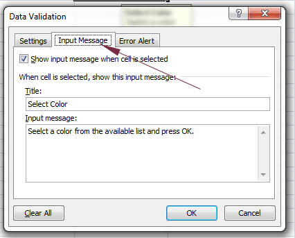
Check the “Show input message when cell is selected” checkbox (if unchecked). Enter the Title and Input message that you want to display as dropdown cell is selected. Press OK.
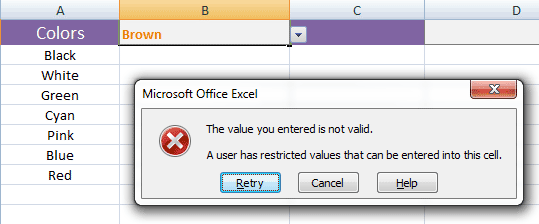
Dealing with error message for incorrect data
Normally, a user may enter any text in a cell where dropdown is created. For example, in our Color dropdown, a user may enter any other color than in the dropdown list. In that case, Excel throws an error by default as shown below:
For customizing this error message, follow these steps.
After creating/selecting the cell containing dropdown, again, go to the Data --> Data Validation and open its dialog.
Press the “Error Alert” Tab and check the “Show error alert if invalid data is entered” (this is done by default).
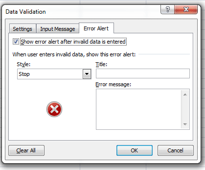
You may customize the style, enter Title and Error message. The style will display the Stop, Warning or Information icon. Use this as per the scenario.
See a customized error message below:
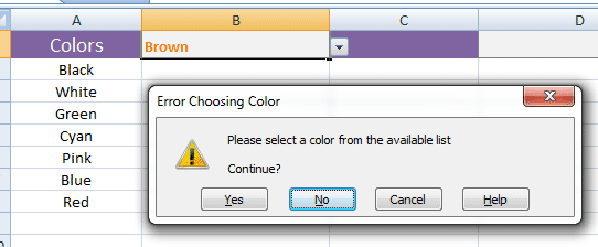
You can see, Brown color does not exist in the dropdown list. So, the Excel displayed a custom error with “Info” icon.
See dropdown in action with HLOOKUP function
Now let us look at the usage of dropdown value for some “real” stuff. In the example, I have an excel sheet containing marks of the students for three subjects and their total.
A user may search the marks of individual subjects and their total for a student. For the subjects and total, I have created a dropdown. As a user selects an option from the dropdown list (placed in C8 cell), the marks are updated automatically in the C12 cell where HLOOKUP formula is used as follows:
=HLOOKUP(C8,A1:E5,2,FALSE)
See the dropdown and updated result in excel sheet:
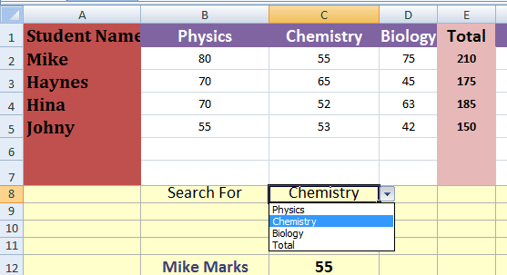
As you select any other option in the dropdown list, the marks will update accordingly.
Using two dropdowns with a formula example
Let us make things a little more complex for using the two dropdown values in a formula. Extending the above example, there was a limitation that it only searched the marks of Student name Mike.
In this type of situation, you may also require letting the user selecting subject and student name so you may search the entire excel sheet.
For that, I have inserted another dropdown that lists student names from the column A i.e (A2:A5). The Search for subject/total dropdown remains the same as in above example.
So, you may now select the subject/total in the first dropdown.
Select the student name from the second dropdown.
The C12 cell displays the marks for the selected subject or total for that student.
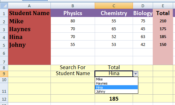
The student name dropdown is created as follows:
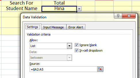
The selected value of this dropdown is used in the MATCH function to locate the row reference in MATCH function. The complete formula used in the C12 cell is:
=HLOOKUP(C8,A1:E5,MATCH(C9,A1:A5,0),FALSE)
You may download this working two-dropdown sheet here.
The example of using dropdown in VLOOKUP function
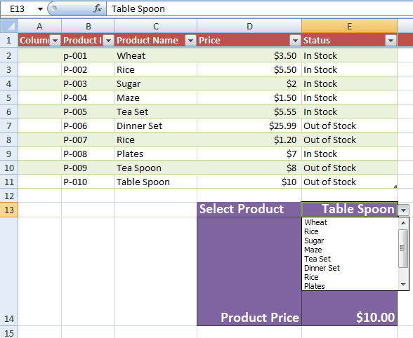
The following example shows using the dropdown value in VLOOKUP function. We have a Product table that contains Product ID, name, price, and status.
As a product is selected from the dropdown list, its price is displayed by using the VLOOKUP function as follows:
The VLOOKUP formula:
=VLOOKUP(E13,C2:E11,2,FALSE)
Where E13 value is taken from the dropdown list.
The price as I selected “Table Spoon” from the dropdown list:
You may get download this excel sheet here.
For learning more about VLOOKUP, go to its tutorial: VLOOKUP function in Excel